Bladeless Turbines: The Full Research Trail
The question that drove the work
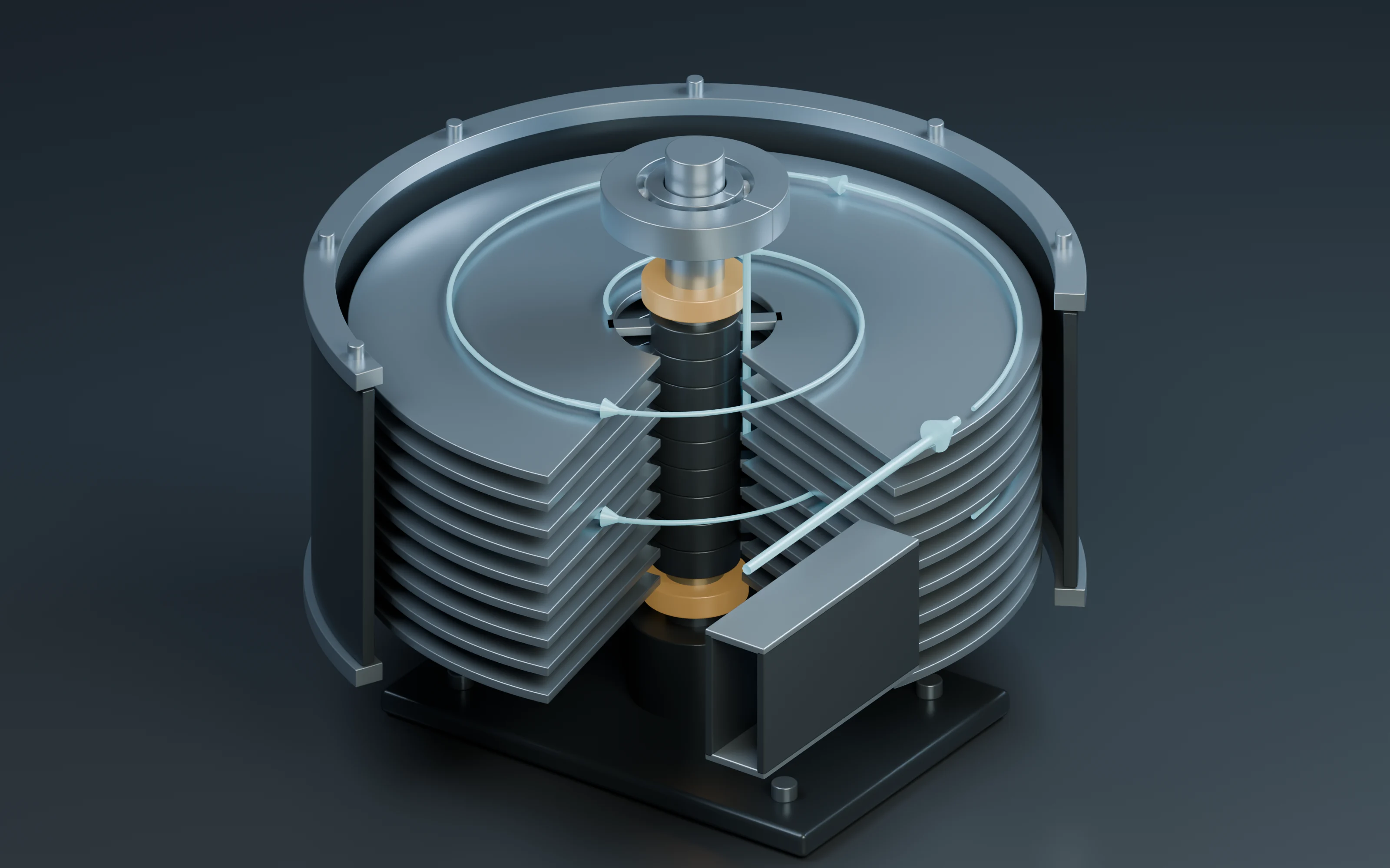
A Tesla turbine transfers energy from a moving fluid to a stack of discs through viscous interaction with their surfaces. A shaft can therefore receive torque without conventional blades. The interesting question is not simply whether the discs can turn. It is how gap, size, flow, losses, speed and stored rotational energy interact, and which of those relationships can actually be established from the available evidence.
This research began with two tempting intuitions: narrower gaps should improve coupling, and a geometrically enlarged machine should behave like the smaller one. Both proved incomplete. The work then developed a residence-time criterion, tried to confront it with published experiments, designed a controlled comparison when the needed data were missing, and explored competing losses. Two surviving seventh-round accounts pursue different extensions: one derives startup and useful-power conditions; the other audits a published experiment's energy balance and electrical units. Both belong to the record.
The calculations below are analytical or synthetic unless explicitly attributed to an external experiment. They are presented together with their assumptions, numerical results, tests and changes of direction. No new physical turbine was built in these rounds.
1. How the machine works and what must be defined
A bladed turbine extracts energy through a flow field shaped by blades. In the disc-machine concept investigated here, viscous shear couples the fluid to disc surfaces. That distinction does not remove the need for an energy source, a pressure/enthalpy budget, or a load that absorbs useful shaft power. The standalone seventh-round account checked the disc-and-viscosity description against Tesla's original turbine patent.
Several quantities must be kept separate throughout the argument:
- Torque, in N·m, is the turning action on the shaft.
- Angular speed, ω, is in rad/s. A speed of n rpm means ω = 2πn/60.
- Shaft power is torque times angular speed. A large torque at zero speed produces no shaft power at that instant.
- Rotational energy, Jω²/2, is energy already stored in a rotating assembly. Its units are joules, not watts.
- Volumetric flow, Q, is in m³/s; mass flow is in kg/s. Neither is an efficiency.
- Pressure drop, Δp, must be distinguished from an inlet pressure reported without a reference convention.
- Efficiency requires a specified useful output and a specified input-energy rate. An algebraic index or a normalized flow cannot stand in for that definition.
The working models deliberately vary in scope. The first is a stationary water channel. Later examples use air, rotating-disc similarity, a dimensionless resistance network and an idealized shaft-torque law. Results can be carried between them as questions or mechanisms, but their numerical parameters do not describe one common experimental machine.
2. Round 1A: narrowing the gap under two different constraints
Starting intuition
The first exploration asked: “If a narrower gap strengthens viscous interaction, must it improve the machine?” Rather than assert an optimum turbine gap, it tested the intuition in a simpler problem where the flow law is explicit.
The proxy was steady, laminar flow of an incompressible Newtonian fluid between fixed parallel plates. It omitted rotor motion, radial geometry and the actual inlet/nozzle. Its purpose was to expose an operating-constraint trade-off before making a turbine-performance claim.
Assumptions and equation
The example used water-like properties and a rectangular channel:
- Dynamic viscosity μ = 0.001 Pa·s
- Density ρ = 1,000 kg/m³
- Channel width b = 0.1 m
- Channel length L = 0.1 m
- Fixed pressure difference Δp = 100 Pa
- Gaps h = 0.2, 0.4 and 0.8 mm
For the ideal wide parallel-plate channel,
Q = b h³ Δp / (12 μ L).
This gives two different experimental questions:
- With pressure difference fixed, how much fluid passes through?
- With flow fixed, how much pressure difference is required?
Numerical results
The fixed-flow reference was the flow at a 0.4 mm gap and 100 Pa.
| Gap | Flow at 100 Pa | Mean velocity | Approximate hydraulic Reynolds number | Pressure required for the reference flow |
|---|---|---|---|---|
| 0.2 mm | 6.6667 × 10⁻⁸ m³/s | 0.003333 m/s | 1.3333 | 800 Pa |
| 0.4 mm | 5.3333 × 10⁻⁷ m³/s | 0.013333 m/s | 10.6667 | 100 Pa |
| 0.8 mm | 4.2667 × 10⁻⁶ m³/s | 0.053333 m/s | 85.3333 | 12.5 Pa |
At fixed pressure, doubling the gap increases this model's flow eightfold. At fixed flow, halving the gap requires eight times the pressure difference. All three approximate hydraulic Reynolds numbers are below 100, an internal check consistent with the chosen laminar proxy.
Test, counterargument and change in question
The saved calculation checked the eightfold fixed-pressure flow ratio, the eightfold fixed-flow pressure penalty, and the three low-Reynolds-number cases. These checks establish the internal arithmetic of the chosen proxy. They do not test a rotating turbine.
The useful correction was to the original intuition: “stronger shear coupling” and “adequate flow with tolerable pressure loss” are competing concerns. Narrowing the gap cannot be judged independently of what the inlet system holds fixed.
The next question became: should an optimization compare fixed inlet kinetic energy, fixed flow or fixed pressure difference? That unresolved choice remained relevant when inlet losses were added in Round 6.
The historical references for this branch were a parallel-plate flow derivation and a 2026 turbine engineering review.
3. Round 1B: why geometric scaling is not dynamic similarity
A second early branch
A separate early full-round package asked whether doubling disc radius while preserving geometric proportions would preserve efficiency. This was the actual parent question cited by Round 2. It is retained alongside the first gap calculation, rather than silently substituting one early account for the other.
The necessary scale check used the rotational Reynolds number:
Re_rot = ρ ω R² / μ = ω R² / ν,
where R is disc radius and ν = μ/ρ is kinematic viscosity.
Calculation
The illustrative air properties were ρ = 1.2 kg/m³ and μ = 1.8 × 10⁻⁵ Pa·s. With R = 0.05 m and a speed of 6,000 rpm:
- Reference rotational Reynolds number: 104,719.76
- Radius doubled to 0.10 m at the same speed: 418,879.02
- Radius doubled and speed reduced to 1,500 rpm: 104,719.76
Thus doubling radius at fixed speed multiplies Re_rot by four. To preserve this one parameter, speed must fall to one quarter.
What was rejected
Geometric similarity alone does not establish dynamic similarity. Even holding Re_rot constant does not establish equal efficiency: gap-to-radius ratio, inlet conditions, leakage, pressure ratio and structural constraints still matter.
This is a narrower conclusion than “the larger machine must be less efficient” or “the efficiencies must differ.” Neither direction nor size of an efficiency change was calculated. The test instead defeats an argument that equal efficiency follows automatically from proportional dimensions.
The branch also referred to a 2022 experimental paper to motivate separating simulated performance from measurements on a specified apparatus. Round 2 developed that distinction further.
4. Round 2: the Reynolds–Mach conflict
Question inherited from the scaling branch
Could speed alone be adjusted to preserve both rotational Reynolds number and disc-edge Mach number when radius changes?
For fixed fluid properties and fixed sound speed c:
Re_rot ∝ ωR²,
M_tip = ωR/c ∝ ωR.
If radius is multiplied by a factor λ, preserving Re_rot requires ω_new/ω_old = λ⁻², whereas preserving M_tip requires ω_new/ω_old = λ⁻¹.
For λ = 2, the required speed factors are 0.25 and 0.50. Except for the zero-speed degenerate case, one speed setting cannot satisfy both requirements for a doubled radius under these assumptions.
Numerical and external evidence
The saved test recorded the radius factor of two, both speed factors, and the incompatibility. The research card separately reported a maximum efficiency of 14.2% ± 0.4 percentage points at 3 barg and 4,000 rpm from the 2022 experimental study.
That reported measurement is an external experimental anchor. It is not the output of the scaling calculation, and it is not an efficiency ceiling for every Tesla turbine. Simulation values discussed elsewhere in the same paper cannot automatically be paired with it as if they were measurements of the same machine under identical conditions.
Counterargument that refined the result
The algebra is exact for the stipulated scaling, but its engineering importance depends on the operating regime. A Mach-number mismatch matters differently when compressibility is negligible than when it materially changes the flow. Reynolds and Mach numbers are also not a complete similarity description.
The next evidence request therefore became more concrete: collect pressure ratio, flow, mechanical output, disc gap, uncertainty and the efficiency definition for the same apparatus. Comparing a small collection of headline percentages would not answer that question.
5. Round 3: momentum diffusion versus residence time
Why add a time scale?
The prior rounds compared size and speed, but had not asked how long fluid remains between the discs. A wider gap gives momentum a greater distance to diffuse across. Whether viscous interaction has time to act depends on residence time as well as geometry.
The round introduced a dimensionless index:
I = ν t / g².
Here g is a physical gap in metres, t is residence time in seconds and ν is kinematic viscosity in m²/s. Equivalently, I compares residence time with the characteristic diffusion time g²/ν. It is a diagnostic index, not a proposed efficiency equation.
Three explicit checks
With ν = 1.5 × 10⁻⁵ m²/s, g = 0.001 m and t = 0.02 s:
- Baseline: I = 0.30
- Double the gap to 0.002 m, keeping time fixed: I = 0.075
- Double the gap and increase time to 0.08 s: I returns to 0.30
The original program checked all three results. The scaling is quadratic: at fixed viscosity and target index, doubling gap requires four times the residence time.
What the calculation changed
“Larger gap allows more flow” was no longer an adequate standalone description. The wider passage also changes the time-distance relationship for viscous coupling. However, this calculation did not determine how actual residence time varies with flow, nor did it include pressure, swirl, rotor speed, thermal effects or compressibility.
The next question was empirical: could this index even rank losses or efficiencies across different gaps on one rotor? That was the task carried into Round 4.
6. Round 4: trying to test the index against published gap experiments
The evidence sought and the evidence found
The target was a within-rotor gap series: the same turbine tested at several gaps under comparable conditions. The recorded literature search identified a 2021 experimental paper whose abstract described adjustable gaps and two prototype diameters.
The research package recorded:
- Prototype diameters: 11.25 cm and 15 cm
- Reported optimum gap: 0.9 mm
- Reported associated pressure: approximately 103.89 kPa
- Maximum efficiencies reported for the two prototypes: 33% and 50%
- Individual same-condition gap-series values available from the abstract: no
The original record did not establish a complete pressure-reference convention or extract the detailed efficiency definitions. Those omissions matter before these figures are normalized into a benchmark.
A calculation near the reported gap
The model was re-evaluated using g = 0.9 mm, ν = 1.5 × 10⁻⁵ m²/s and t = 0.02 s:
I = 0.37037037.
Alternatively, setting a target I = 0.30 gives:
- At g = 0.9 mm: required t = 0.0162 s
- At g = 1.8 mm: required t = 0.0648 s
The factor-of-four time requirement survives the change of gap values. These are model calculations; the required times were not measured in the paper.
The wrong turn that was explicitly rejected
The two reported maximum efficiencies cannot be treated as two points on a single rotor's gap-response curve. They belong to different prototypes. Without the per-gap observations, comparable operating conditions and residence-time measurements, the abstract does not validate I as an efficiency-ranking rule.
This round therefore did not close the empirical test proposed in Round 3. It located a relevant experiment and exposed exactly which observations were missing. The proposed next step was to obtain the full within-machine curves, or to specify the minimum measurement design if those values could not be obtained.
7. Round 5: the 36-run measurement design
Turning a data gap into a controlled comparison
Round 5 produced a factorial plan rather than claiming that the absent experimental data had appeared. The design crossed:
- Two rotor diameters: 11.25 and 15 cm
- Three physical gaps: 0.6, 0.9 and 1.2 mm
- Two pressure settings: 70 and 104 kPa
- Three repeats per combination
The total was 2 × 3 × 2 × 3 = 36 planned observations. The saved matrix enumerated all combinations; it did not contain measured outcomes.
Complete condition schedule
Each row below represents three planned repeated measurements.
| Diameter | Gap | Pressure setting | Planned repeats |
|---|---|---|---|
| 11.25 cm | 0.6 mm | 70 kPa | 1, 2, 3 |
| 11.25 cm | 0.6 mm | 104 kPa | 1, 2, 3 |
| 11.25 cm | 0.9 mm | 70 kPa | 1, 2, 3 |
| 11.25 cm | 0.9 mm | 104 kPa | 1, 2, 3 |
| 11.25 cm | 1.2 mm | 70 kPa | 1, 2, 3 |
| 11.25 cm | 1.2 mm | 104 kPa | 1, 2, 3 |
| 15 cm | 0.6 mm | 70 kPa | 1, 2, 3 |
| 15 cm | 0.6 mm | 104 kPa | 1, 2, 3 |
| 15 cm | 0.9 mm | 70 kPa | 1, 2, 3 |
| 15 cm | 0.9 mm | 104 kPa | 1, 2, 3 |
| 15 cm | 1.2 mm | 70 kPa | 1, 2, 3 |
| 15 cm | 1.2 mm | 104 kPa | 1, 2, 3 |
Eight required raw-data fields
The original design specified torque in N·m, rpm, inlet pressure in Pa, outlet pressure in Pa, mass flow in kg/s, gas temperature in K, measured gap in mm and uncertainty.
Those fields would permit a much better comparison than pairing peak efficiencies from different machines. In particular, a nominal spacer size is not a substitute for a measured gap, and a pressure setting is not a substitute for recording both ends of the device.
The design's stated aim was to separate gap and diameter effects and reduce load-related confusion. A remaining weakness is that load was not an explicit factor in the enumerated matrix, nor did the matrix prescribe a full load-control protocol. The reconstruction therefore treats load matching, pressure convention and measurement timing as details still to be specified, not as controls already demonstrated by the 36 slots.
The saved calculation also retained the diffusion-index prediction that doubling gap from 0.6 to 1.2 mm at fixed residence time reduces I to one quarter. That is a proposed model comparison for future data, not a result from the planned measurements.
Outcome
The experiment became concrete enough to discuss quantities and comparisons, but remained unexecuted. The next research priority was still to obtain comparable published curves before resorting to new hardware. No procurement or bench-test campaign was necessary to continue the analytical work.
8. Round 6: competition between disc-gap and inlet losses
Why the first gap law was insufficient
The initial channel law gave Q ∝ h³ at fixed pressure. A turbine system also has an inlet or nozzle, and increasing passage capacity does not remove that other restriction. Round 6 asked how much the gap-only prediction changes when an additional loss term shares the pressure budget.
It used a synthetic, dimensionless series-resistance model:
ΔP = q/g³ + βq².
In this equation, q and ΔP are normalized flow and pressure drop; g is gap divided by the minimum reference gap. This g is not the physical metre-valued gap used directly in the diffusion index. β is a stipulated quadratic inlet/nozzle-loss coefficient.
Solution and assumptions
For ΔP = 1, the model combines a linear-in-flow gap loss and a quadratic-in-flow inlet loss. Writing a = 1/g³:
- If β = 0: q = 1/a = g³
- If β > 0: q = [−a + √(a² + 4β)]/(2β)
The program evaluated g = 1, 1.5 and 2 at β = 0, 1 and 4.
| β | q at g = 1 | q at g = 1.5 | q at g = 2 | Flow ratio, g = 2 versus g = 1 |
|---|---|---|---|---|
| 0 | 1.000000 | 3.375000 | 8.000000 | 8.000000 |
| 1 | 0.618034 | 0.862766 | 0.939451 | 1.520064 |
| 4 | 0.390388 | 0.464333 | 0.484619 | 1.241377 |
Tests and interpretation
The saved executable explicitly asserted that the zero-nozzle-loss case reproduces an eightfold flow increase and that the β = 1 case gives less than a twofold increase. All nine tabulated values were saved as model outputs.
The result explains why the first cubic law cannot identify an optimum turbine gap. When another restriction takes a significant share of the pressure budget, widening the gap produces a much smaller increase in total flow. The larger β cases are counterexamples to carrying the isolated-channel eightfold result into a whole system without checking the inlet.
This still does not calculate shaft power. Torque, rotor speed, compressibility and measured values of β are absent. Even a correct flow model would require an additional energy-transfer model before it could predict useful output or efficiency.
The next evidence target was a within-rotor curve set at two pressures, enabling inlet resistance to be distinguished from gap resistance. The records do not show that these curves were obtained.
9. Round 7A: startup and a useful-power envelope
Two seventh-round branches
The surviving standalone Round 7 research card and the Round 7 bundled package contain different substantive studies. Both identify the same preceding Round 6 result. There is no basis in the recovered record for treating them as interchangeable or for claiming that one definitively superseded the other.
This section preserves the standalone startup/power branch. The next section preserves the bundled energy/unit-audit branch. Their equations address complementary questions, but they were not jointly fitted to a measured turbine.
The startup question
A disc can receive fluid torque and still fail to start if resisting torque is too large. The standalone branch used a simple model consisting of viscous driving, speed-dependent resistance and a fixed friction term.
The following expanded notation makes the card's reported result explicit:
- Ω: effective angular speed associated with the driving fluid
- ω: shaft angular speed, constrained to forward operation, ω ≥ 0
- k: positive fluid-to-disc coupling coefficient
- b: nonnegative speed-dependent resistance coefficient
- τ₀: nonnegative fixed resisting torque
The model's driving torque is k(Ω − ω), with additional resistance bω + τ₀. The torque available to a useful load is therefore
τ_available(ω) = kΩ − τ₀ − (k + b)ω.
The associated useful-power envelope is
P(ω) = [kΩ − τ₀]ω − (k + b)ω².
This is an explanatory reconstruction of the algebra summarized in the card. The archived standalone test artifact was not recovered with the bundled evidence used here, so the card's reported checker is not represented as a separately inspected test run.
Startup boundary and optimum
At rest, forward net driving torque is kΩ − τ₀. Self-starting in this simplified model requires
kΩ > τ₀.
When that condition holds, the power curve is a downward-opening parabola. Its maximum occurs at
ω* = (kΩ − τ₀) / [2(k + b)],
with
P_max = (kΩ − τ₀)² / [4(k + b)].
The zero-useful-load endpoint is ω₀ = (kΩ − τ₀)/(k + b), so the modeled maximum-power point lies at half that endpoint speed.
The important counterexample
The squared expression for P_max is not valid on its own. If kΩ ≤ τ₀, the unconstrained stationary point occurs at zero or negative speed. It is outside the positive-running regime when the inequality is strict. Over the allowed forward-speed domain, the maximum available power is zero at ω = 0.
Thus the complete model result is piecewise:
- kΩ > τ₀: positive startup margin and the interior maximum above
- kΩ ≤ τ₀: no positive available-power operating point; maximum available power is zero
Blindly squaring a negative startup margin would manufacture a positive power result for a rotor that the model cannot drive forward. Catching that boundary failure was the substantive correction.
Energy-budget check
The coupling constants and effective fluid speed need evidence-based identification. In addition, the predicted power must fit within the input-energy rate. For a suitable incompressible pressure-driven approximation, ΔpQ provides a pressure-work budget. For a steam or other compressible-flow application, the appropriate enthalpy-flow accounting is needed instead; the simple pressure-times-volume-flow expression cannot be applied indiscriminately.
The next step named by this branch was to constrain parameters with existing fluid data. It did not require a purchased turbine before the startup algebra could be investigated.
10. Round 7B: inertia, transient energy and a unit discrepancy
The published experiment behind the question
The bundled Round 7 changed focus to a 2026 experimental article. It asked whether a reported advantage of steel discs over aluminum discs could be explained by greater inertia, by temporary stored energy, by different fluid conditions, or by ambiguity in electrical units.
The recorded reading scope was the public article's HTML text: geometry, methods, loaded-speed results and current-unit wording. Readable numerical pixels from Table 2 and Figure 11 were not acquired in that round.
The dimensions recorded from the paper were ten discs, 150 mm diameter, 1 mm thickness and a 10 mm shaft. The calculation treated the discs as uniform annuli with an inner radius of 5 mm. It used assumed material densities of 7,800 kg/m³ for steel and 2,700 kg/m³ for aluminum, and excluded shaft and generator inertia.
Reconstructed mass, inertia and stored energy
For n uniform annular discs with outer radius R, inner radius r and thickness h:
m_total = nπ(R² − r²)hρ,
J_discs = ½m_total(R² + r²),
E_rot = ½J_discsω².
The reported loaded speeds recorded for the 10-bar setting were 3,440 rpm for steel and 2,155 rpm for aluminum.
| Quantity | Steel-disc scenario | Aluminum-disc scenario |
|---|---|---|
| Assumed density | 7,800 kg/m³ | 2,700 kg/m³ |
| Total modelled mass of ten discs | 1.372248 kg | 0.475009 kg |
| Modelled disc inertia | 0.00387660 kg·m² | 0.00134190 kg·m² |
| Recorded loaded speed | 3,440 rpm | 2,155 rpm |
| Calculated stored rotational energy | 251.533 J | 34.170 J |
| Approximate output power recorded from the text | 22 W | 11 W |
| Energy at that power for a chosen 10 s interval | 220 J | 110 J |
The last row is an illustrative integration interval selected by the research, not a duration established as the paper's test protocol. The mass values are totals for the ten-disc stack; the original output field's abbreviated wording must not be mistaken for the mass of one disc.
Why inertia cannot by itself explain sustained output
The rotational balance is
J dω/dt = τ_fluid − τ_load − τ_loss.
Multiplying by ω gives the energy-rate balance:
d(½Jω²)/dt = P_fluid − P_load − P_loss,
for constant J.
At steady speed, dω/dt = 0. Inertia then provides no continuing extra power term. A heavier rotor can store more energy and affect acceleration or deceleration, but “it is heavier” is not by itself an explanation for a larger sustained output at constant speed.
During a transient, stored energy must be included explicitly. The calculated steel stack's 251.5 J and the illustrative 220 J over ten seconds show why one must distinguish a time-integrated output from a snapshot of rotor energy. They do not establish how much energy was discharged during any actual run. The fluid may continue supplying power, the rotor may change speed, and the model omits other rotating components.
The result therefore ruled out an insufficient explanation rather than diagnosing the actual cause of the reported material difference.
The electrical-unit check
The record transcribed approximate power/current wording as 22 W with 0.9 mA for steel, and 11 W with 0.55 mA for aluminum. If each pair were simultaneous values in a context where P = VI applies, literal conversion of the stated milliamps gives:
- Steel: 22/(0.9 × 10⁻³) = 24,444.44 V
- Aluminum: 11/(0.55 × 10⁻³) = 20,000 V
For comparison only, interpreting the current numbers as amperes would give 24.44 V and 20 V. That alternative is a hypothesis about the discrepancy, not a correction to the article.
The calculation cannot decide whether the unit is mistyped, whether the values refer to different operating points, or whether additional measurement details explain the pairing. It also does not establish misconduct. The appropriate next evidence is the original voltage/current data, confirmation of simultaneous sampling, and the steady or transient conditions of the reported output.
11. What the successive corrections established
The research moved forward by replacing broad intuitions with narrower questions that could be tested:
- “Narrower must be better.” The fixed-channel proxy revealed a cubic pressure/flow trade-off. The operating constraint has to be stated before choosing a direction of optimization.
- “A larger geometric copy behaves the same.” The rotational Reynolds number changes by four when radius doubles at fixed speed. Geometry alone does not establish similarity.
- “Fix Reynolds number and the problem is solved.” Reynolds and tip-Mach preservation demand different speed scalings under fixed fluid conditions.
- “The fluid has enough contact because the gap is small.” A residence-time versus diffusion-time comparison supplied a specific index and a fourfold time penalty for doubling gap.
- “Two published efficiency numbers validate the gap model.” The numbers belonged to different prototypes. The required within-machine curve was still missing.
- “A measurement matrix is already evidence.” The 36 conditions defined a possible experiment, but supplied no measured outcome. Load control remained to be made explicit.
- “The channel's eightfold flow gain is the system gain.” Adding a quadratic inlet loss reduced the doubling-gap gain to 1.52 or 1.24 in the synthetic cases.
- “The square in the optimum-power formula guarantees output.” A nonpositive startup margin puts the formal optimum outside the feasible running domain.
- “More inertia explains more sustained power.” The inertia term vanishes at steady speed. Transient energy and continuing energy transfer must be separated.
- “An implausible unit pairing can be silently repaired.” The electrical check preserves the literal unit and identifies the clarification needed.
These are the results of the research process: explicit scaling laws, model counterexamples, a measurement design, a constrained power envelope and an energy/unit audit. They form a more useful account than one isolated optimum-speed formula, while keeping the unresolved empirical questions visible.
12. Technical appendix: equations, assumptions and verification record
A. Variable and unit conventions
| Symbol | Meaning | Units or convention |
|---|---|---|
| μ | Dynamic viscosity | Pa·s |
| ν | Kinematic viscosity, μ/ρ | m²/s |
| ρ | Density | kg/m³ |
| h, g in physical-gap equations | Channel or disc gap | m |
| g in Round 6 | Gap divided by a reference gap | Dimensionless |
| Q | Physical volumetric flow | m³/s |
| q | Normalized flow in Round 6 | Dimensionless |
| Δp | Physical pressure difference | Pa |
| ΔP in Round 6 | Normalized pressure difference | Dimensionless |
| R, r | Outer and inner radius | m |
| ω, Ω | Shaft and effective driving angular speeds | rad/s |
| t | Residence or elapsed time, specified by context | s |
| J | Moment of inertia | kg·m² |
| τ₀ | Fixed resisting torque in the startup model | N·m |
| k, b | Torque-per-angular-speed coefficients | N·m·s/rad |
| β | Quadratic loss coefficient in normalized model | Dimensionless |
The symbol b denotes channel width in Round 1A and resistance coefficient in Round 7A. They are unrelated quantities despite sharing a letter. Likewise, the physical gap and normalized gap must not be substituted into each other's equations without conversion.
B. Derivation details
For the channel proxy, mean velocity is U = Q/(bh). The recorded approximate hydraulic Reynolds number uses hydraulic diameter D_h ≈ 2h, appropriate to the wide-slot approximation: Re_h ≈ ρU(2h)/μ. Substituting the flow law explains the tabulated sensitivity to gap.
For the scaling branch, fixed fluid properties give Re_new/Re_old = (ω_new/ω_old)(R_new/R_old)². Tip Mach instead scales with the first power of radius. Equating both ratios to one leads directly to the conflicting speed requirements for any nontrivial radius change.
For the diffusion index, holding I fixed gives t = Ig²/ν. The quarter-index and quadruple-time results are the same algebra viewed under different controlled variables.
For the resistance model, solving βq² + aq − ΔP = 0 with a = g⁻³ gives the positive root. The historical code used the direct quadratic formula. An algebraically equivalent form, q = 2ΔP/[a + √(a² + 4βΔP)], avoids cancellation when the two terms in the direct numerator are close. This alternative is an explanatory numerical observation, not an additional archived test.
For the startup model, define A = kΩ − τ₀ and B = k + b > 0. Then P = Aω − Bω², dP/dω = A − 2Bω, and d²P/dω² = −2B. If A > 0, the stationary point is a maximum in the forward-speed domain. If A ≤ 0, dP/dω ≤ 0 for every ω ≥ 0 and the maximum is P(0) = 0. This constrained optimization is the reason the startup branch must be stated piecewise.
For the inertia calculation, the annular-disc formula gives the inertia of the modeled stack only. Incorporating a shaft, coupling, generator, holes, spacers or a nonuniform mass distribution would require additional geometry or measurements.
C. What the original checks actually checked
| Stage | Available check or result | What it establishes |
|---|---|---|
| Initial gap branch | Two eightfold ratios; all three Re_h values below 100 | Arithmetic and internal regime consistency of the stationary channel proxy |
| Scaling branch | Re_rot values at two radii and two speeds | Fixed-fluid rotational-Reynolds scaling |
| Round 2 | Speed factors 1/4 and 1/2 | Incompatibility of the two stipulated similarity requirements |
| Round 3 | I = 0.30, I = 0.075, restoration by fourfold time | Diffusion-index arithmetic |
| Round 4 | Reported gap recorded; fourfold time scaling; absent gap series explicitly recorded | A bounded literature extraction and a model recalculation |
| Round 5 | Enumerated 36-condition matrix and eight fields | Completeness of the planned factor combinations, not execution |
| Round 6 | Nine normalized flow values; assertions for the 8× and less-than-2× cases | Behavior of the chosen two-loss synthetic model |
| Standalone Round 7 | Card reports a theoretical checker and startup-boundary correction | Card-supported analytical result; companion test artifact not inspected here |
| Bundled Round 7 | Mass/inertia/energy and literal-unit calculations saved with assumptions | Numerical consequences of the recorded dimensions, speeds and assumed densities |
The historical programs and saved results were inspected for this reconstruction. The complete multi-topic research pipelines were not rerun. A program flag such as “PASS” or “check: true” is interpreted according to the local assertion it accompanies, not as independent validation of a turbine design or every statement in a cited paper.
13. Public references and the remaining evidence gaps
The original rounds used the following public references. This page preserves their role in the historical work; it does not present a new independent reading of every full paper.
- Tesla's turbine patent, US1061206A: disc-machine mechanism cited by the standalone startup branch.
- Parallel-plate flow derivation: theoretical background for the initial fixed-channel proxy.
- 2026 engineering review: initial literature context for gaps, inlets, fluids and losses.
- 2022 experimental study: the recorded 14.2% ± 0.4-percentage-point measurement and the need to distinguish simulation from specified apparatus data.
- Additional Energies reference retained in Round 2: contextual reference; the recovered card did not attach a separate quantitative result to it.
- 2021 adjustable-gap study: the recorded two diameters, 0.9 mm optimum and separate prototype maxima. Its needed within-machine curves were not recovered by the original gap-model rounds.
- 2026 experimental evaluation: source of the geometry, loaded speeds and power/current wording recorded by the energy-audit branch; the necessary table/figure numbers remained incompletely read.
Three empirical gaps remain central. First, a comparable gap series is needed before the diffusion or resistance models can be judged against a rotor. Second, the startup envelope needs identified coupling/loss parameters and an input-energy budget. Third, the material comparison needs simultaneous voltage/current records and a time-resolved distinction between steady output and changing rotational energy.
Those gaps do not erase the calculations already established. They specify exactly what observation would turn each analytical result into a stronger performance model.