Six positions, seven states: an exact graph and its readable atlas
What this report establishes
This is a documented finite graph model, not a newly discovered mathematical theory, a physical simulation, or an inference about an external system. The existing generator and its saved arrays were inspected and exhaustively checked. They implement the six-fold Cartesian product of the cycle graph C7, written here as C7 □ C7 □ C7 □ C7 □ C7 □ C7. The symbol □ matters: an unqualified “graph power” could mean a different operation.
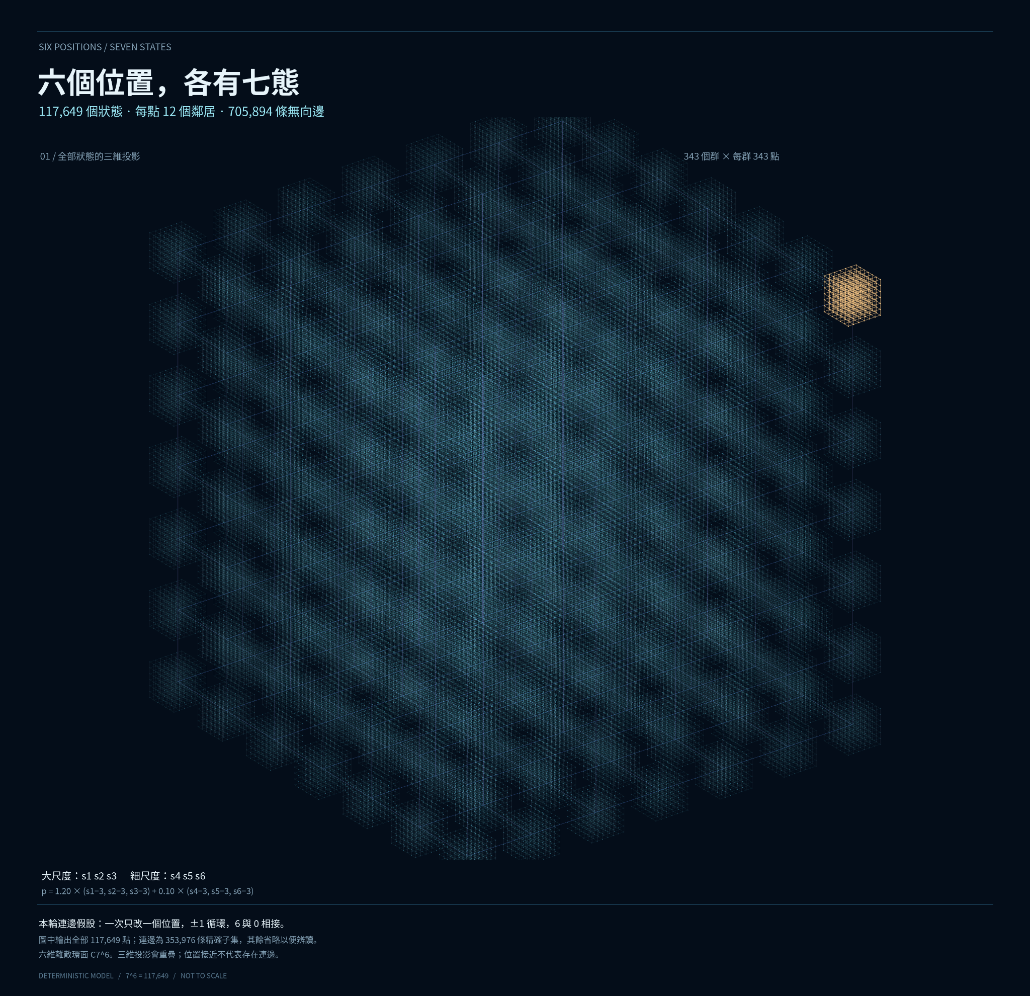
There are 117,649 vertices, degree 12 at every vertex, and 705,894 distinct undirected edges. All state identities and all edges remain in complete-graph.npz. The new drawings separate the graph from its placement on a page: no fog, depth of field, lighting, denoising, or material shading is used.
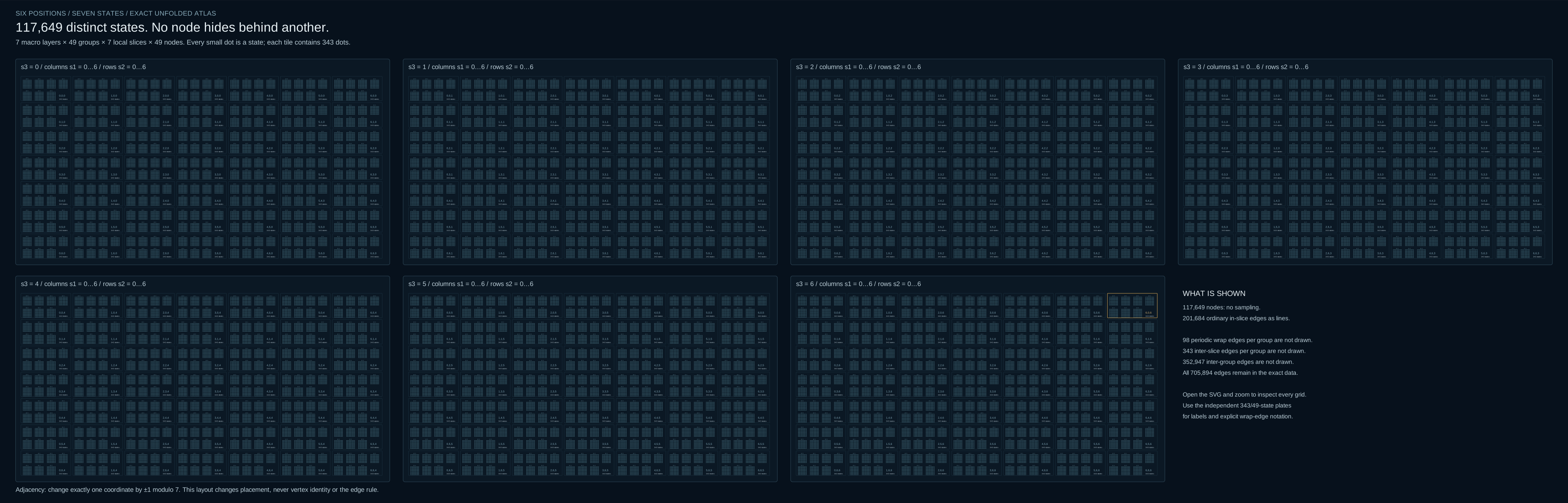
The primary overview, overview-all-states.svg, contains all 117,649 node instances, arranged without depth occlusion. It is not a replacement of the state set by a few large cells. The additional overview-layers.svg is explicitly a group-address index. Neither overview claims to display every edge.
1. State set and an independently chosen adjacency relation
Let V = {0,1,2,3,4,5,6}^6. A state is s=(s1,s2,s3,s4,s5,s6). Therefore |V|=7^6=117,649.
Seven possible values alone do not imply a circular ordering, nearest-neighbour transitions, or an edge from 6 back to 0. Those are modelling choices. Here the values are treated as residues modulo 7, and distinct s,t are adjacent exactly when there is one index k such that:
- tj=sj for every j≠k;
- tk−sk is congruent to +1 or −1 modulo 7.
Thus 0 connects to 1 and 6. Changing 0 directly to 3 is not an edge. A different application could choose a path, a complete graph, a directed transition rule, or a rule inferred from data; it would be a different graph on the same state set.
This definition agrees with the standard Cartesian graph-product rule: one coordinate moves along an edge of its factor graph while all other coordinates remain fixed. NetworkX: Cartesian product. The factor is a cycle, whose first and last vertices are joined. NetworkX: cycle graph.
2. What the actual generator does
The existing build_c7.py enumerates itertools.product(range(7), repeat=6). It assigns the original global integer ID
id(s) = s1·7^5 + s2·7^4 + s3·7^3 + s4·7^2 + s5·7 + s6, from 0 to 117,648.
For each coordinate k and each state i, the saved edge array contains the positive cyclic step. If sk<6, its endpoint is i+7^(6−k); if sk=6, it is i−6·7^(6−k). Thus it generates 6·7^6 positive-step pairs. These pairs represent undirected edges: each cycle edge is generated once, not twice. Negative steps are recovered by undirected incidence.
The verification does not assume that these intended formulas match the file. It reads the saved NPY arrays from the NPZ using the Python standard library and compares every state, every endpoint, every projected position and every selected-edge index with independently regenerated values. It also rejects loops and duplicate unordered pairs and counts incidence at every vertex.
3. Counts, distances, and the graph family
For each of six coordinates there are two distinct neighbours (+1 and −1). Different coordinates cannot produce the same neighbour. Hence deg(s)=6·2=12. By counting edge endpoints, 2|E|=|V|·12, so |E|=117,649·6=705,894. There are 117,649 edges for each changed coordinate.
The graph is connected because coordinates can be adjusted one at a time around their cycles. The graph distance is
d(s,t) = Σ(k=1..6) min(|sk−tk|, 7−|sk−tk|).
Each coordinate requires at least its cycle distance, and adjusting the coordinates separately attains that sum. The diameter is therefore 6·3=18. These are consequences of this chosen graph, not experimental findings.
| Model | Per-coordinate graph | Vertices | Degree | Undirected edges |
|---|---|---|---|---|
| This model | C7, six factors | 117,649 | 12 | 705,894 |
| Seven-symbol Hamming graph H(6,7) | K7, six factors | 117,649 | 36 | 2,117,682 |
| Binary hypercube Q6 | K2, six factors | 64 | 6 | 192 |
In H(6,7), any change to a different symbol in exactly one coordinate is allowed, giving 6·(7−1)=36 neighbours. This differs from restricting that coordinate to its two cycle neighbours. The standard Hamming-graph definition connects tuples at Hamming distance one. SageMath: HammingGraph.
For example, (0,0,0,0,0,0) and (3,0,0,0,0,0) have Hamming distance 1 but distance 3 in the present graph. The supplied Q6 illustration is a different 64-vertex graph; it is not evidence that the seven-state model is a binary hypercube. No Menger-sponge deletion rule occurs in this generator.
4. The original spatial placement: 343 groups of 343 states
The generator assigns the three-dimensional position
p(s)=1.2·(s1−3,s2−3,s3−3)+0.1·(s4−3,s5−3,s6−3).
Fixing the first three coordinates gives 7^3=343 groups. Each group contains the 7^3=343 choices of the final three coordinates. Group centres are separated by 1.2 along each relevant axis, while each local point cloud spans 0.6 along each axis. Adjacent group bounding boxes therefore have a gap of 0.6. This scale choice helps identify groups; it is not a graph metric or a physical length.
Injectivity in 3D. If two positions agree, then in each coordinate 12Δa+Δb=0, with Δb in {−6,…,6}. A nonzero Δa would make |12Δa|≥12, which Δb cannot cancel. Thus Δa=Δb=0 in all three coordinates. Every state has a distinct 3D point. Enumeration confirms 117,649 unique positions.
This does not give an injective 2D image. The earlier orthographic camera looks along (12,−18,11). For the integer coordinates P=10p, equal pairs (18Px+12Py, 11Px−12Pz) identify the same ideal projected point. Previous exact counting gave 83,517 distinct projected positions: 60,319 vertices participate in multiply occupied positions, with at most five depth layers. Finite line width creates further visual overlap. This is a consequence of that camera placement, not a requirement to collapse states in every drawing.
5. Exact induced subgraphs
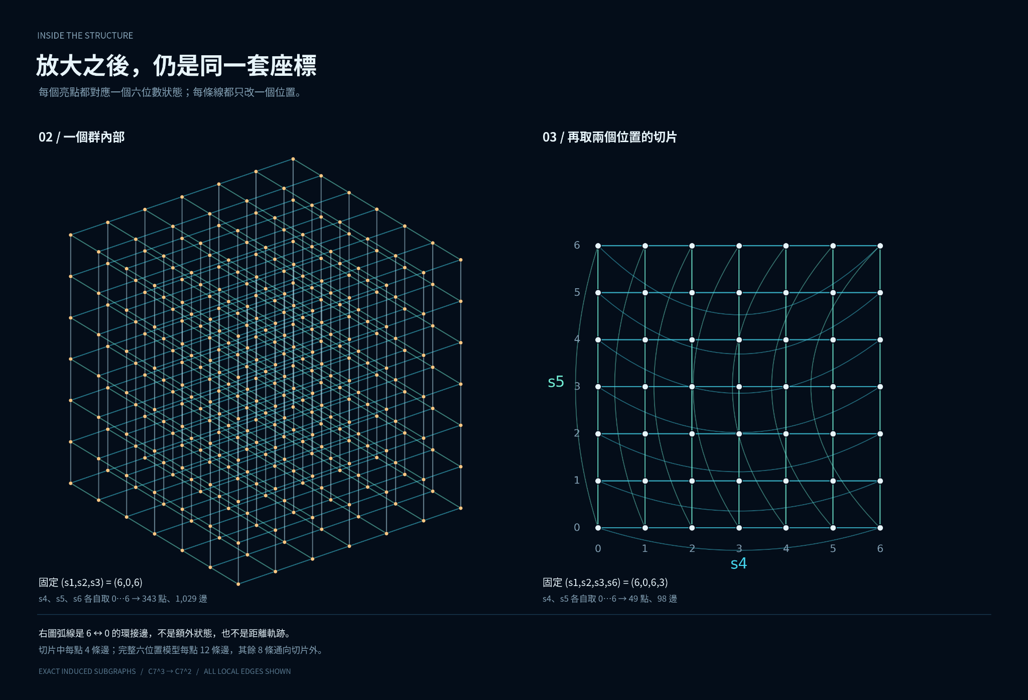
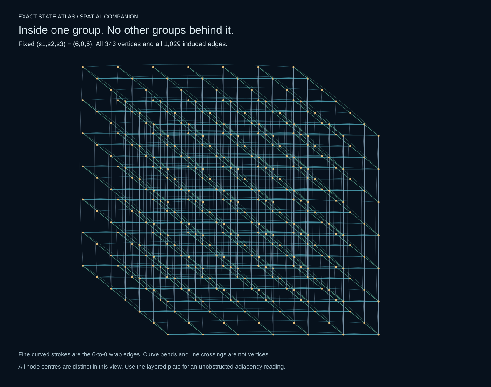
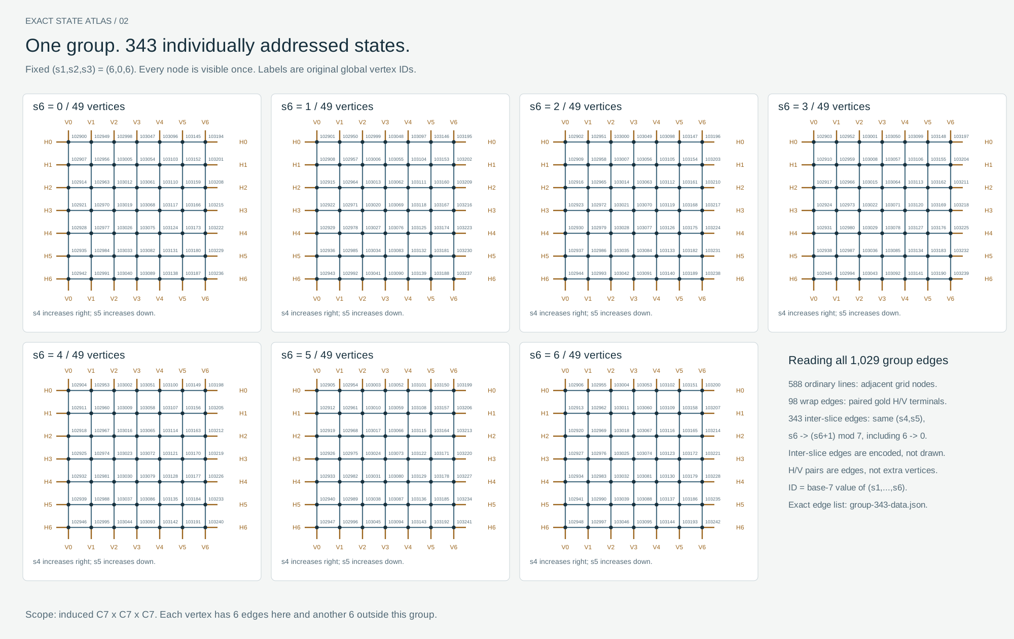
Fix (s1,s2,s3)=(6,0,6). The remaining graph is C7 □ C7 □ C7: 343 vertices, degree 6 internally, and 343·6/2=1,029 edges. Each vertex has six additional edges to other groups in the full six-factor graph. Those are outside the induced group, not missing internal edges.
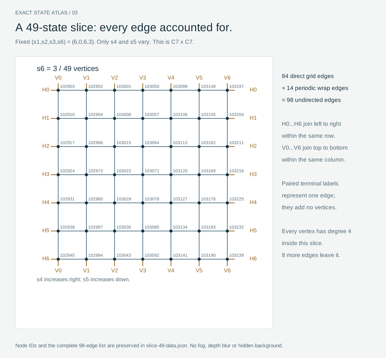
Fix s6=3 as well. The remaining slice is C7 □ C7: 49 vertices, internal degree 4, and 49·4/2=98 edges. Its other eight incident edges leave the slice. All 49 global IDs and all 98 endpoint pairs are saved in slice-49-data.json; the 343-state counterpart is group-343-data.json.
6. What each drawing includes and omits
| Asset | Vertices represented | Edge representation |
|---|---|---|
overview-all-states.svg | All 117,649, once each | 201,684 ordinary in-slice lines; remaining edges explicitly omitted visually |
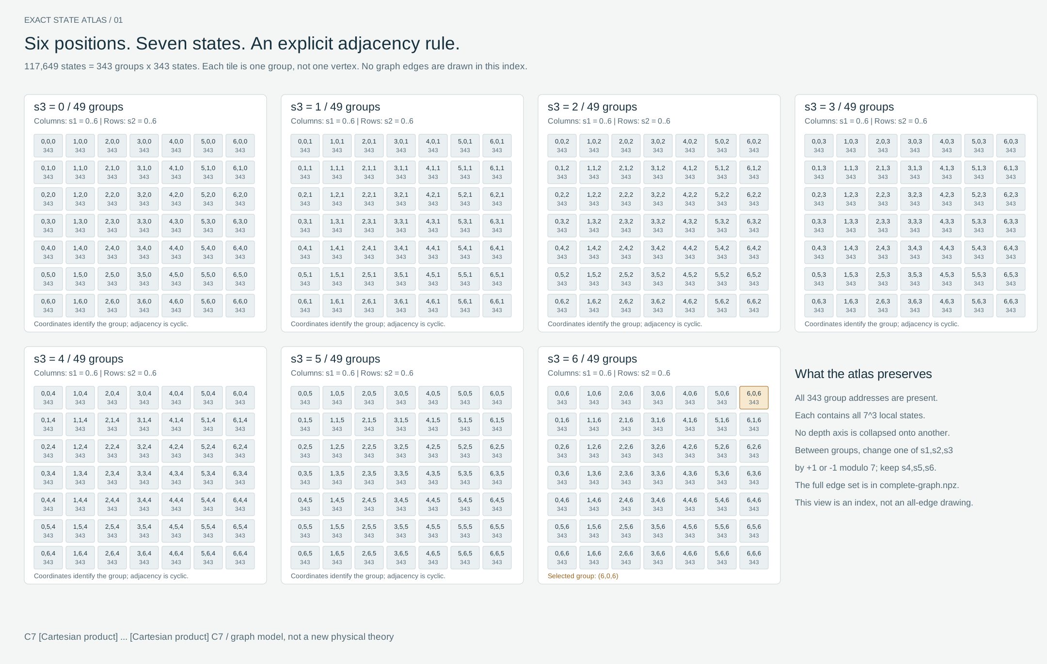
overview-layers.svg | 343 group tiles, each standing for 343 states | Address index; no graph edges |
group-343.svg | All 343, once each, across seven s6 panels | 588 ordinary lines; 98 wrap edges through paired terminals; 343 cross-panel edges given by the exact matching-coordinate rule and edge list |
slice-49.svg | All 49, once each | 84 ordinary lines + 14 wrap edges through paired terminals = all 98 edges |
group-343-spatial.svg | All 343 distinct projected node centres | All 1,029 edges as lines/curves; crossings remain possible, but no background groups |
The dense overview arranges seven s3 layers. Each layer contains a 7×7 grid of group addresses (s1,s2); each group contains seven disjoint s6 panels; each panel contains a 7×7 grid of (s4,s5). There is no node sampling. Its omitted edges are 33,614 in-slice wraps, 117,649 between local s6 panels, and 352,947 between groups. Together with the 201,684 drawn edges, these total 705,894. Layout rearrangement does not create or delete graph edges.
In the labelled plates, H0…H6 pair the left and right boundary nodes of the same row; V0…V6 pair top and bottom boundary nodes of the same column. A paired terminal encodes one periodic edge. Terminals are not vertices. Across s6 panels, matching (s4,s5) coordinates connect c to (c+1) mod7, including panel 6 to panel 0. This encodes 7·49=343 edges without long lines passing through other panels. The plates are not claimed to be crossing-free drawings of every edge as one continuous stroke.
Every node in the independent plates has its original global ID in SVG metadata; the readable layered plate also prints the ID. Dense SVG instances carry the macro coordinates and local coordinates hierarchically. Their ID is recovered by the same base-7 formula. The reusable SVG geometry reduces file size; it does not reduce the number of represented states.
The earlier Blender selection is retained for audit: all 352,947 within-group edges plus 1,029 between-group edges at local coordinates (3,3,3), total 353,976, about 50.1458% of the full graph. Its count matches the reference caption, but the reference's original selection code was unavailable, so equality of the two selected sets is not established. It must never be captioned “all relationships shown.”
7. Why the supplied references look clearer
The newly supplied originals were downloaded and visually inspected. Their actual raster dimensions are: Q6 1638×2048, C7 global 2048×1980, and C7 local detail 2048×1394. None needs to exceed the Blender main image's 3200×2000 to read more clearly.
The references use a uniform dark field, restrained thin strokes, distinct node marks, and separate global and local explanations. The original local panel isolates one group and a two-coordinate slice. The Blender detail instead retained all background groups, so enlarging the camera also enlarged their interference. The Blender main local tube diameter was approximately 0.25 pixels at the output resolution, and its 32-sample denoising could smooth subpixel structure. No actual fog or depth-of-field blur was enabled. The reference global view still has central overlap; it does not prove that every state is separately readable in one flat projection.
The revised SVGs preserve arbitrarily scalable geometry. Raster overview images are navigation previews: no finite small screen can make 117,649 labelled vertices simultaneously legible. Readers should open/zoom the full SVG and use the isolated group and slice plates for inspection. The labelled plates use 2.2-unit line widths (over two pixels at native size), a uniform background and no denoising. The dense atlas intentionally requires vector zoom for its smallest marks.
8. Actual verification and limitations
verification.json records successful exhaustive comparisons with the saved original arrays: state ordering, all 705,894 edge endpoints, uniqueness, no loops, degree 12, all projected positions, all selected-edge indices, and the 343/49 induced subgraphs. dense-atlas-verification.json checks 343 disjoint group rectangles and the exact number of displayed node instances. svg-verification.json records unique local node IDs, distinct centres, and validity of every directly drawn endpoint pair; the check also verifies both terminals of each periodic edge. The checked original NPZ SHA-256 is included in the verification record; a hash verifies byte identity, not scientific truth.
The new generator uses Python's standard library; NetworkX and SageMath documentation were consulted for definitions but neither library was installed or run as an independent graph implementation. Counts and injectivity are supported by explicit proofs plus exhaustive checks, not by a visual impression. The supplied screenshots do not reveal the original reference rendering code or camera exactly.
All SVGs and PNGs were generated locally in the authorised task workspace. No website was modified or deployed. The old artistic renders remain available but are no longer the recommended precise main illustration. The public-ready report and assets contain no private source IDs, account information, signed links or local-user paths.
Reproducibility and scope
Run build_precise.py, then build_dense.py, then build_spatial_group.py from the task directory. These scripts read the existing exact NPZ and write the c7-precise assets. rsvg-convert rasterizes the SVG geometry without a 3D rendering engine. The accompanying JSON files are the authoritative endpoint lists for the local plates; the NPZ contains the complete graph. Changes in page placement, lighting style or line routing do not imply a new graph theorem or empirical mechanism.